Here is a somewhat unconventional recommendation for the design of online experiments:
Set your default parameters for alpha (α) and beta (β) to the same value.
This implies that you incur equal cost from a false positive as from a false negative. I am not suggesting you necessarily use these parameters for every experiment you run, only that you set them as the default. As humans, we are inescapably influenced by default choices1, so it is worthwhile to pick a set of default risk parameters that most closely match the structure of our decision-making. A default of symmetric risk—setting α=β—has a beneficial side effect of making experiment design easier to understand and communicate. A more parsimonious and intuitive process is more likely to actually get performed the next time someone is in your org is planning an experiment.
Why sample size calculations actually matter
Performing a sample size calculation is the most important first step you can take to ensure your experiment is successful. The calculation itself acts as a forcing function2, requiring us to ask ourselves a number of questions which reduce our chances of succumbing to common post-analysis pitfalls such as underpowered tests or the multiple comparisons problem.
- What is the specific metric we will use to measure success of this experiment?
- What magnitude of effect do we expect to see? Are changes on the scale of 1% or 100%?
- What level of risk are we willing to accept of being wrong?
Unfortunately, many people consider this calculation to be optional. In many companies, there is nothing truly blocking people from starting an experiment without a plan. So in the interest of efficiency and 80/20, many teams end up embracing a defacto test-first, analyze-second strategy. Besides making us vulnerable to the post-analysis pitfalls mentioned above, this unfortunately also reduces our capacity to learn from experiments. The beauty of the scientific method is that when we make falsifiable hypotheses and proceed to falsify them, we are then presented with golden opportunity to refactor our mental models of the world. We can use data to refine our intuitions. But if we don’t actually write out a crisp hypothesis before starting the experiment, it is too easy to victim to hindsight bias, subconciously rewriting the narrative into one which affirms our identity but denies us personal growth.
A very brief review of Type I & II errors
Without diving too deep here, recall that there are two key parameters which correspond to the two ways we can make a mistake in the context of a statistical test:
- alpha (α) represents our long-run accepted risk of false positives (FPR).
- beta (β) represents our long-run accepted risk of false negatives (FNR).
- The power of a statistical test is its ability to correctly identify a true effect (1-β)
I will defer to Google’s ML Crash Course for deeper understanding on this topic, since it provides the clearest learning example I’ve seen using a “boy who cried wolf” analogy.
The problem with your typical sample size calculation
The typical sample size calculation is a trade-off between three parameters: α, β, and the minimum detectable effect (MDE), which is the smallest relative change in our metric of interest which is meaningful to us.
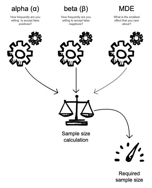
Required sample size is a function of three input parameters.
This calculation is straightforward if we have predetermined inputs and merely want to know the output. But this does not match the reality of planning an experiment in a tech company. It is more of a negotiation than a calculation, particularly when working with a non-technical stakeholder. A typical conversation around sample size might look like this:
- PM asks for your help planning an experiment for a new feature they are launching.
- You calculate the required sample size based on their primary KPI and send it back.
- PM replies asking if you accidentally meant days where you wrote X weeks duration.
- You explain the nature of the calculation, false positives, false negatives, etc.
- PM probes for where he or she can apply the good ol’ 80-20 rule to achieve results more quickly.
This conversation can be frustrating for many analysts, but essentially what your stakeholder is trying to do here is to develop an intuition for what the marignal cost of each parameter is, so that they can discern where to compromise. This is a process which is a bit clumsy when we’ve got three “knobs” to work with. When we set α=β, we effectively eliminate one of these knobs, and turn it into a two-dimensional problem involving MDE and risk. At this point, we can summarize the required sample size at various levels of each using a data table a 2D plot. Conceptually, we can visualize the trade-off between these three parameters in a similar fashion to the project management triangle.
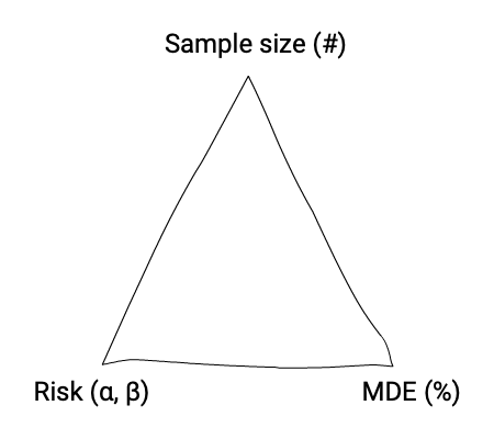
Any change in one dimension requires sacrifice in one of the other two.
Question your defaults (α=0.05, β=0.20)
The first page of google results consists largely of medicore sample size calculators pretending to be easy-to-use by simply hiding α and β parameters. The better ones—including my personal favourite, Evan Miller’s Sample Size Calculator—set default values and provide clear explanations as to what these parameters mean. And yet, every calculator which does display α and β—including Evan’s and other ones—set their default values to α=0.05 and β=0.20.
If you don’t have have a particularly strong opinion—or understanding—of what your relative ratio between these types of risk should be, it is tempting to simply go with the default options. Before you do so, allow me the opportunity to disabuse you of the notion that these are sacred numbers, unanimously agreed upon by some group of clever statisticians sitting in some room years ago.
Significance
There has been a decent amount of media coverage recently around the problems with p-values3 and their role in the social sciences replication crisis. So naturally at least a few peope have asked Why is 0.05 such a sacred number?
The use of the 5% p-value threshold appears to have become universal in biomedical research, yet it does not seem to to be based on any clear statistical reasoning. So far as I can make out, the origin of this threshold seems to lie in a discussion of the theoretical basis of experimental design, published by the Cambridge geneticist and statistician RA Fisher in 1926.
— Origin of the 5% p-value threshold [BMJ]
The short answer: it isn’t. But even though there is nothing a priori special about p <0.05, one could make a solid argument that the practice of having a generally-agreed-upon benchmark is the important part. A shared standard is valuable when we want to compare levels of evidence across different studies or research groups. which standardizes the level of evidence used across different research groups.
Power
The practice of planning experiments with 80% power is an equally accepted standard, but it does not seem to be discussed nearly as often. It also raises the question: why are these defaults set at a 4:1 ratio?
Although there are no formal standards for power (sometimes referred to as π), most researchers assess the power of their tests using π = 0.80 as a standard for adequacy. This convention implies a four-to-one trade off between β-risk and α-risk. (β is the probability of a Type II error, and α is the probability of a Type I error; 0.2 and 0.05 are conventional values for β and α).
— Power (statistics) [Wikipedia]
I suspect that this assymetry in risk is at least partially due to the close connection between the development of statistics and the biomedical space. Suppose you are a statistician working for a pharma company. You are running an experiment to determine whether a potential new drug is more effective at treating a particular ailment than an exiting alternative. In this context, a false negative—failing to detect that the new drug is in fact more effective—could mean aborting development and missing out on the potential profit from bringing it to market. A false positive—incorrectly concluding the new drug is more effective when it is the same or worse—could mean spending billions of dollars to bring an ineffective drug to market, then subsequently spending billions more on with lawsuits and reputational damage in the decade that follows. In this hypothetical high-stakes scenario in which we face assymetric costs, it is prudent to be extra-conservative on false positives (α) at the expense of increased false negatives (β).
Flavours of hypothesis testing: Fisher vs. Neyman–Pearson
So it seems entirely plausible that particular domains—including biomedical research—require an assymetric risk profile, in which we value one of false positives or negatives more heavily than the other. But why do we never see scenarios in which we value false negatives more highly than false positives? While there are in fact a few such studies4, they are few and far between. Alexander Etz lays out a good argument for why this is the case, in his article Question: Why do we settle for 80% power? Answer: We’re confused.:
Why do they not adjust α and settle for α = 0.20 and β = 0.05? Why is small α a non-negotiable demand, while small β is only a flexible desideratum? A large α would seem to be scientifically unacceptable, indicating a lack of rigor, while a large β is merely undesirable, an unfortunate but sometimes unavoidable consequence of the fact that observations are expensive or that subjects eligible for the trial are hard to find and recruit. We might have to live with a large β, but good science seems to demand that α be small.
A lot of the confusion around hypothesis testing seems to stem from the fact that it is a blend of two underlying philosophies: Fisherian significance testing, and Neyman–Pearson hypothesis testing. It is particularly difficult to grok for outsiders, because while these two paradigms have irreconcilable differences, they also share some simliarities, and even use the same terminology of null hypotheses, alpha, etc.
I will defer to this excellent explanation of the differences by StackExchange user “gong”:
Fisher thought that the p-value could be interpreted as a continuous measure of evidence against the null hypothesis. There is no particular fixed value at which the results become ‘significant’.
On the other hand, Neyman & Pearson thought you could use the p-value as part of a formalized decision making process. At the end of your investigation, you have to either reject the null hypothesis, or fail to reject the null hypothesis.
The Fisherian and Neyman-Pearson approaches are not the same. The central contention of the Neyman-Pearson framework is that at the end of your study, you have to make a decision and walk away.
One particularly frustrating pieces of statistical terminology—“failing to reject the null hypothesis”—comes from the Fisherian paradigm. If you are evaluating evidence in relation to a single hypothesis and you do not achieve a significant result, it could be either because such a result is not possible—the null hypothesis is correct—or simply because you did not collect enough data to disprove it. Therefore in a Fisherian context, we cannot accept a hypothesis, we can only fail to reject it.
This paradigm is a natural match for the decentralized structure of scientific discovery in society. Hypotheses aren’t evaluated only once, so false negatives only delay discovery, rather than eliminating it. But researchers face implicit pressure to find surprising (significant) results for their experiment. Funding for future research may depend on it. Since it is not quite as sexy to fund experiments that verify knowledge we already “know”5, it makes sense to be very conservative with false positives, at the cost of accepting more false negatives.
This paradigm is less good of a match to the typical decision-making context in a modern tech company in which A/B testing is being performed. We are not interested in advancing the societal body of shared scientific knowledge. We just want to make optimal decisions in an environment of uncertainty. Should we launch version A or B? If we truly walk away after making the decision, then failing to reject the null hypothesis is tantamount to accepting it.
The Neyman–Pearson paradigm is a better fit for this scenario, because it pairs statistics with decision theory. In the NP framework, indecision is not an option. There is no option to “collect more data”. We plan a required sample size, collect data, make a binary decision between A and B, and then walk away. Rather than providing some continuous measure of evidence for or against a hypothesis, NP hypothesis testing arms us with the tools to confidently make decisions which minimize our long-run regret.
Unprivilege your null hypothesis
If you are testing two versions of your website, which should you designate as the null hypothesis, and which as the alternative hypothesis? It is standard practice to choose a null hypothesis which reflects the “status quo” that you are attempting to disprove. Given the typical defaults of α=0.05 and β=0.20, this means your null hypothesis occupies a “priviliged” position of being innocent until proven guilty6. But it can be alarming to observe that the outcome (decision) from an experiment can entirely flip depending on how you frame your null hypothesis7. Doesn’t feel particularly objective, does it?
A fantastic side effect of setting α = β when our costs of mistakes are equal is that we can be agnostic as to what our default option is. We don’t have to be as careful as to which hypothesis we designate as null. Consider the following two scenarios:
- You are testing the impact of a new landing page concept on a single market. You have only translated content for a single language, and you’d like to A/B test the new concept before investing in more translations. Unless you see a significant positive effect in your experiment, you plan on staying with the existing system.
- Your backend team has done some major refactoring work, and you’d like to run an A/B test to verify that QA did not overlook any critical bugs. All things equal, you would prefer to go with the new refactored codebase, so you plan on launching the change unless you see a significant negative effect from the experiment.
| Landing page | Refactor | |
|---|---|---|
| Default | Stay with existing version | Launch new version |
| False positive | Wasted resources | Missed opportunity for improved conversion |
| False negative | Missed opportunity for improved conversion | Worse conversion |
These two scenarios share a common failure mode—missed opportunity—but because our default decision differs, our risk is treated differently as well. This failure mode is denoted as β-risk in the first scenario, and α-risk in the second. If we were to use the default parameters (α=0.05, β=0.20) for both experiments, we could say “we planned and ran both experiments the same way” but our chance of missing an opportunity would differ by a factor of 4x. If we use a symmetrical risk profile, then we do not need to pay such close attention to which our default options are, because the long-run risk of making each type of mistake is the same.
A pragmatic approach to statistical rigor
If you are championing statistical thinking and experimentation practices in a move-fast-and-break-things environment, you need to pick your battles. For example: it’s probably not worth kicking up a fuss about people in your org treating confidence intervals like posterior probabilities.
On the other hand, I would argue it is certainly worth encouraging and enabling people to perform sample size calculations as part of a pre-experiment planning process. Such a process has multiple benefits: it reduces the risk of implicit multiple comparisons8 which would inflate your long-run rate of false positives, and also reduces the number of underpowered tests you perform. Underpowered tests in particular can lead to a pernicious scenario in which experiment results lose credibility within the organization. Small simplifications to the planning process such as using a default of α = β can help you achieve this goal.
Although the magnitude of improvement from the “opt-out organ donation” study has been partially debunked, every good salesperson knows there is some power behind the default effect. ↩︎
The biggest value comes not from the output of the calculation, but rather from the questions we must ask ourselves during the process. “Plans Are Worthless, But Planning Is Everything” – Dwight D Eisenhower. ↩︎
800 scientists say it’s time to abandon “statistical significance” (Vox) ↩︎
Justify Your Alpha by Minimizing or Balancing Error Rates (The 20% Statistician) ↩︎
This has changed somewhat since the Replication crisis, but the fact this crisis occured at all indicates there is a systemic bias towards new discoveries. ↩︎
This is anlogous to the legal concept of Presumption of innocence. Priviliging the null hypothesis certainly makes sense here. A criminal escaping justice is unfortunate, but an innocent citizen wrongly imprisoned is horrific. ↩︎
I found a good example in this StackExchange question which illustrates how our decision can flip depending on which hypothesis we assign to be null. ↩︎
Even if you aren’t explicitly testing multiple hypotheses, not having a clearly defined hypothesis before running your experiment leaves you vulnerable to inflated FPR via researcher degrees of freedom. ↩︎