Goal
A few weeks ago while learning about Naive Bayes, I wrote a post about implementing Naive Bayes from scratch with Python. The exercise proved quite helpful for building intuition around the algorithm. So this is a post in the same spirit on the topic of AdaBoost.
Who is Ada, anyways?
Boosting refers to a family of machine learning meta-algorithms which combine the outputs of many “weak” classifiers into a powerful “committee”, where each of the weak clasifiers alone may have an error rate which is only slightly better than random guessing.
The name AdaBoost stands for Adaptive Boosting, and it refers to a particular boosting algorithm in which we fit a sequence of “stumps” (decision trees with a single node and two leaves) and weight their contribution to the final vote by how accurate their predictions are. After each iteration, we re-weight the dataset to assign greater importance to data points which were misclassified by the previous weak learner, so that those data points get “special attention” during iteration $t+1$.
How does it compare to Random Forest?
| Property | Random Forest | AdaBoost |
|---|---|---|
| Depth | Unlimited (a full tree) | Stump (single node w/ 2 leaves) |
| Trees grown | Independently | Sequentially |
| Votes | Equal | Weighted |
The AdaBoost algorithm
This handout gives a good overview of the algorithm, which is useful to understand before we touch any code.
A) Initialize sample weights uniformly as $w_i^1 = \frac{1}{n}$.
B) For each iteration $t$:
- Find weak learner
$h_t(x)$which minimizes$\epsilon_t = \sum_{i=1}^n \mathbf{1}[h_t(x_i) \neq y_i] \, w_i^{(t)}$. - We set a weight for our weak learner based on its accuracy: $\alpha_t = \frac{1}{2} \ln \Big( \frac{1-\epsilon_t}{\epsilon_t} \Big)$
- Increase weights of misclassified observations: $w_i^{(t+1)} = w_i^{(t)} \cdot e^{-\alpha^t y_i h_t(x_i)}$.
- Renormalize weights, so that $\sum_{i=1}^n w_i^{(t+1)}=1$.
C) Make final prediction as weighted majority vote of weak learner predictions: $H(x) = \text{sign} \Big( \sum_{t=1}^T \alpha_t h_t(x) \Big)$.
Getting started
Helper plot function
We’re going to use the function below to visualize our data points, and optionally overlay the decision boundary of a fitted AdaBoost model. Don’t worry if you don’t understand everything that is happening here, it is not critical to understanding the algorithm itself.
from typing import Optional
import numpy as np
import matplotlib.pyplot as plt
import matplotlib as mpl

def plot_adaboost(X: np.ndarray,
                  y: np.ndarray,
                  clf=None,
                  sample_weights: Optional[np.ndarray] = None,
                  annotate: bool = False,
                  ax: Optional[mpl.axes.Axes] = None) -> None:
    """ Plot ± samples in 2D, optionally with decision boundary """

    assert set(y) == {-1, 1}, 'Expecting response labels to be ±1'

    if not ax:
        fig, ax = plt.subplots(figsize=(5, 5), dpi=100)
        fig.set_facecolor('white')

    pad = 1
    x_min, x_max = X[:, 0].min() - pad, X[:, 0].max() + pad
    y_min, y_max = X[:, 1].min() - pad, X[:, 1].max() + pad

    if sample_weights is not None:
        sizes = np.array(sample_weights) * X.shape[0] * 100
    else:
        sizes = np.ones(shape=X.shape[0]) * 100

    X_pos = X[y == 1]
    sizes_pos = sizes[y == 1]
    ax.scatter(*X_pos.T, s=sizes_pos, marker='+', color='red')

    X_neg = X[y == -1]
    sizes_neg = sizes[y == -1]
    ax.scatter(*X_neg.T, s=sizes_neg, marker='.', c='blue')

    if clf:
        plot_step = 0.01
        xx, yy = np.meshgrid(np.arange(x_min, x_max, plot_step),
                             np.arange(y_min, y_max, plot_step))

        Z = clf.predict(np.c_[xx.ravel(), yy.ravel()])
        Z = Z.reshape(xx.shape)

        # If all predictions are positive class, adjust color map acordingly
        if list(np.unique(Z)) == [1]:
            fill_colors = ['r']
        else:
            fill_colors = ['b', 'r']

        ax.contourf(xx, yy, Z, colors=fill_colors, alpha=0.2)

    if annotate:
        for i, (x, y) in enumerate(X):
            offset = 0.05
            ax.annotate(f'$x_{i + 1}$', (x + offset, y - offset))

    ax.set_xlim(x_min+0.5, x_max-0.5)
    ax.set_ylim(y_min+0.5, y_max-0.5)
    ax.set_xlabel('$x_1$')
    ax.set_ylabel('$x_2$')
Generate a fake dataset
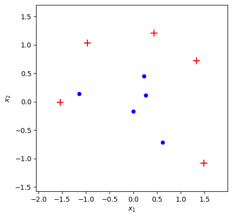
We will generate a toy dataset using a similar approach to sklearn documentation but using less data points. The key here is that we want to have two classes which are not linearly separable, since this is the ideal use-case for AdaBoost.
from sklearn.datasets import make_gaussian_quantiles
from sklearn.model_selection import train_test_split

def make_toy_dataset(n: int = 100, random_seed: int = None):
    """ Generate a toy dataset for evaluating AdaBoost classifiers """

    n_per_class = int(n/2)

    if random_seed:
        np.random.seed(random_seed)

    X, y = make_gaussian_quantiles(n_samples=n, n_features=2, n_classes=2)

    return X, y*2-1

X, y = make_toy_dataset(n=10, random_seed=10)
plot_adaboost(X, y)
Benchmark with scikit-learn
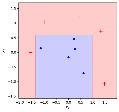
Let’s establish a benchmark for what our model’s output should resemble by importing AdaBoostClassifier from scikit-learn and fitting it to our toy dataset.
from sklearn.ensemble import AdaBoostClassifier

bench = AdaBoostClassifier(n_estimators=10, algorithm='SAMME').fit(X, y)
plot_adaboost(X, y, bench)

train_err = (bench.predict(X) != y).mean()
print(f'Train error: {train_err:.1%}')
Train error: 0.0%

The classifier fully fits the training dataset in 10 iterations, which is not surprising given that the data points in our toy dataset are reasoanbly well separated.
Rolling our own AdaBoost classifier
Below is the skeleton code for our AdaBoost classifier. After fitting the model, we’ll save all the key attributes to the class—including sample weights at each iteration-so we can inspect them later to understand what our algorithm is doing at each step.
The table below shows a mapping between the variable names we will use and the math notation used earlier in the description of the algorithm.
| Variable | Math |
|---|---|
sample_weights with shape: (T, n) | $ w_{i}^{(t)} $ |
stumps with shape: (T, ) | $ h_t(x) $ |
stump_weights with shape (T, ) | $ \alpha_t $ |
errors with shape: (T, ) | $ \epsilon_t $ |
clf.predict(X) | $ H_t(x) $ |
class AdaBoost:
    """ AdaBoost enemble classifier from scratch """

    def __init__(self):
        self.stumps = None
        self.stump_weights = None
        self.errors = None
        self.sample_weights = None

    def _check_X_y(self, X, y):
        """ Validate assumptions about format of input data"""
        assert set(y) == {-1, 1}, 'Response variable must be ±1'
        return X, y
Fitting the model
Recall our algorithm to fit the model:
- Find weak learner
$h_t(x)$which minimizes$\epsilon_t = \sum_{i=1}^n \mathbf{1}[h_t(x_i) \neq y_i] \, w_i^t$. - We set a weight for our weak learner based on its accuracy: $\alpha_t = \frac{1}{2} \ln \Big( \frac{1-\epsilon_t}{\epsilon_t} \Big)$
- Increase weights of misclassified observations: $w_i^{(t+1)} = w_i^{(t)} \cdot e^{-\alpha_t y_i h_t(x_i)}$. Note that $y_i h_t(x_i)$ will evaluate to $+1$ when hypothesis agrees with label, and $-1$ when it does not agree.
- Renormalize weights, so that $\sum_{i=1}^n w_i^{(t+1)} =1$.
The code below is essentially a 1-to-1 implementation of the above, but there are a few things to note:
- Since the focus here is understanding the ensemble element of AdaBoost, we’ll outsource the logic of picking each $h_t(x)$ to
DecisionTreeClassifier(max_depth=1, max_leaf_nodes=2). - We set the initial uniform sample weights outside of the for-loop and set the weights for $t+1$ within each iteration $t$, unless it is the last iteration. We are going out of our way here to save an array of sample weights on the fitted model, so that we can later visualize the sample weights at each iteration.
from sklearn.tree import DecisionTreeClassifier

def fit(self, X: np.ndarray, y: np.ndarray, iters: int):
    """ Fit the model using training data """

    X, y = self._check_X_y(X, y)
    n = X.shape[0]

    # init numpy arrays
    self.sample_weights = np.zeros(shape=(iters, n))
    self.stumps = np.zeros(shape=iters, dtype=object)
    self.stump_weights = np.zeros(shape=iters)
    self.errors = np.zeros(shape=iters)

    # initialize weights uniformly
    self.sample_weights[0] = np.ones(shape=n) / n

    for t in range(iters):
        # fit  weak learner
        curr_sample_weights = self.sample_weights[t]
        stump = DecisionTreeClassifier(max_depth=1, max_leaf_nodes=2)
        stump = stump.fit(X, y, sample_weight=curr_sample_weights)

        # calculate error and stump weight from weak learner prediction
        stump_pred = stump.predict(X)
        err = curr_sample_weights[(stump_pred != y)].sum()# / n
        stump_weight = np.log((1 - err) / err) / 2

        # update sample weights
        new_sample_weights = (
            curr_sample_weights * np.exp(-stump_weight * y * stump_pred)
        )

        new_sample_weights /= new_sample_weights.sum()

        # If not final iteration, update sample weights for t+1
        if t+1 < iters:
            self.sample_weights[t+1] = new_sample_weights

        # save results of iteration
        self.stumps[t] = stump
        self.stump_weights[t] = stump_weight
        self.errors[t] = err

    return self
Making predictions
We make a final prediction by taking a “weighted majority vote”, calculated as the sign (±) of the linear combination of each stump’s prediction and its corresponding stump weight.
$$ H_t(x) = \text{sign} \Big( \sum_{t=1}^T a_t h_t(x) \Big) $$
def predict(self, X):
    """ Make predictions using already fitted model """
    stump_preds = np.array([stump.predict(X) for stump in self.stumps])
    return np.sign(np.dot(self.stump_weights, stump_preds))
Performance
Now let’s put everything together, and fit the model with the same parameters as our benchmark.
# assign our individually defined functions as methods of our classifier
AdaBoost.fit = fit
AdaBoost.predict = predict

clf = AdaBoost().fit(X, y, iters=10)
plot_adaboost(X, y, clf)

train_err = (clf.predict(X) != y).mean()
print(f'Train error: {train_err:.1%}')
Train error: 0.0%
Success! We’ve achieved the exact same result as our sklearn benchmark. I cherry-picked this toy dataset to show the strengths of AdaBoost, but you can run this notebook yourself and see that it matches the output regardless of starting conditions.
Developing intuition
Visualizing our learner step-by-step
Since we saved all intermediate variables as arrays to our fitted model, we can use the function below to visualize how our ensemble learner evolves at each iteration $t$:
- The left column shows the “stump” weak learner selected, which corresponds to $h_t(x)$.
- The right column shows the cumulative strong learner so far: $H_t(x)$.
- The size of the data point markers reflects their relative weighting. Data points misclassified in the previous iteration will be more heavily weighted—and therefore appear larger—in the next iteration.
def truncate_adaboost(clf, t: int):
    """ Truncate a fitted AdaBoost up to (and including) a particular iteration """
    assert t > 0, 't must be a positive integer'
    from copy import deepcopy
    new_clf = deepcopy(clf)
    new_clf.stumps = clf.stumps[:t]
    new_clf.stump_weights = clf.stump_weights[:t]
    return new_clf


def plot_staged_adaboost(X, y, clf, iters=10):
    """ Plot weak learner and cumulaive strong learner at each iteration. """

    # larger grid
    fig, axes = plt.subplots(figsize=(8, iters*3),
                             nrows=iters,
                             ncols=2,
                             sharex=True,
                             dpi=100)

    fig.set_facecolor('white')

    _ = fig.suptitle('Decision boundaries by iteration')
    for i in range(iters):
        ax1, ax2 = axes[i]

        # Plot weak learner
        _ = ax1.set_title(f'Weak learner at t={i + 1}')
        plot_adaboost(X, y, clf.stumps[i],
                      sample_weights=clf.sample_weights[i],
                      annotate=False, ax=ax1)

        # Plot strong learner
        trunc_clf = truncate_adaboost(clf, t=i + 1)
        _ = ax2.set_title(f'Strong learner at t={i + 1}')
        plot_adaboost(X, y, trunc_clf,
                      sample_weights=clf.sample_weights[i],
                      annotate=False, ax=ax2)

    plt.tight_layout()
    plt.subplots_adjust(top=0.95)
    plt.show()

clf = AdaBoost().fit(X, y, iters=10)
plot_staged_adaboost(X, y, clf)
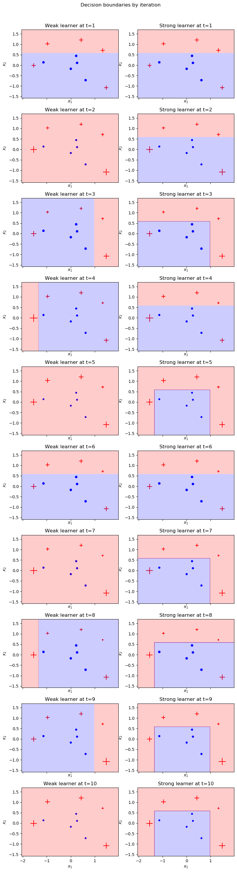
Why do some iterations have no decision boundary?
You may notice that our weak learners at iterations $t=2,5,7,10$ classify all points as positive. This occurs because given the current sample weights, the lowest error is achieved by simply predicting all data points to be positive. Note that in each of the plots above for these iterations, the negative samples are surrounded by proportially higher-weighted positive samples.
There is no way to draw a linear decision boundary to correctly classify any number of negative data points without misclassifying a higher cumulative weight of positive samples. This does not stop our algorithm from converging though. All the negative points are misclassified and therefore increase in sample weight. This updating of weights allows the next iteration’s weak learner to discover a meaningful decision boundary.
Why do we use that specific formula for alpha_t?
Are you curious why we use this particular value for $\alpha_t$? We can show that the choice of $a_t = \frac{1}{2} \ln \Big( \frac{1-\epsilon_t}{\epsilon_t} \Big)$ minimizes exponential loss $L_{exp}(x, y) = e^{-y \, h(x)}$ over the training set.
Ignoring the sign function, our strong learner $H$ at iteration $t$ is a weighted combination of weak learners $h(x)$. At any given iteration $t$, we can define $H_t(x)$ recursively as its value at iteration $t-1$ plus the weighted weak learner of the current iteration.
$$ \begin{aligned} H_t(x) &= \sum_{i=1}^t \alpha_i h_i(x) \\ &= H_{t-1} + \alpha_t h_t(x) \end{aligned} $$
Our loss function applied to $H$ is the average loss across all $n$ data points. We can substitute in our recursive definition of $H_t(x)$, and split the exponential term using the identity $e^{a+b}=e^a e^b$.
$$ \begin{aligned} L(H_t) &= \tfrac{1}{n} \sum_{i=1}^n e^{-y_i H_t(x_i)} \\ &= \tfrac{1}{n} \sum_{i=1}^n e^{-y_i H_{t-1}(x_i)} e^{-y_i \alpha_t h_t(x_i)} \\ &= \tfrac{1}{n} \sum_{i=1}^n \color{lightgrey}{e^{-y_i H_{t-1}(x_i)}} e^{-y_i \alpha_t h_t(x_i)} \\ &= \tfrac{1}{n} \sum_{i=1}^n \color{lightgrey}{w^t_i} \; e^{-y_i \alpha_t h_t(x_i)} \\ \end{aligned} $$
Now we take the derivative of our loss function with respect to $\alpha_t$ and set it to zero to find the parameter value at which the loss function is minimized. We can split the summation into two: cases where $h_t(x_i) = y_i$ and cases where $h_t(x_i) \neq y_i$.
$$ \begin{aligned} L(H_t) &= \tfrac{1}{n} \sum_{i=1}^n \color{lightgrey}{w^t_i \,} e^{-y_i \alpha_t h_t(x_i)} \\ \frac{\partial L}{\partial \alpha_t} = 0 &= - \tfrac{1}{n} \sum_{i=1}^n w^t_i \, y_i h_t(x_i) e^{-y_i \alpha_t h_t(x_i)} \\ &= - \tfrac{1}{n} \sum_{i: h_t(x_i) = y_i}^n w^t_i \, e^{-\alpha_t} - \tfrac{1}{n} \sum_{i: h_t(x_i) \neq y_i}^n w^t_i \, e^{\alpha_t} \\ \end{aligned} $$
Finally, we recognize the summation of weights is equivalent to our error calculation discussed earlier: $\sum D_t(i) = \epsilon_t$. Making the substitution and then manipulating algebraically allows us to isolate $\alpha_t$.
$$ \begin{aligned} 0 &= (\epsilon_t-1) e^{-\alpha_t} + \epsilon_t e^{\alpha_t} \\ (1-\epsilon_t) e^{-\alpha_t} &= \epsilon_t e^{\alpha_t} \\ \frac{1 - \epsilon_t}{\epsilon_t} &= \frac{e^{\alpha_t}}{e^{-\alpha_t}} = e^{2 \alpha_t} \\ \alpha_t &= \frac{1}{2} \ln \bigg( \frac{1 - \epsilon_t}{\epsilon_t} \bigg) \end{aligned} $$
Further reading
- sklearn.ensemble.AdaBoostClassifier – Official scikit-learn documentation
- University of Toronto CS – AdaBoost – Understandable handout PDF which lays out a pseudo-code algorithm and walks through some of the math.
- Weak Learning, Boosting, and the AdaBoost algorithm – Discussion of AdaBoost in the context of PAC learning, along with python implementation.
- AdaBoost: Implementation and intuition – Python implementation with visualization function, served partially as the inspiration for this post.