One textbook which is frequently recommended on Hacker News threads about self-study math material is Blitzstein and Hwang’s An Introduction to Probability. Having just recently finished the book, I realized that this is the first textbook I have truly worked through end-to-end while studying a topic outside a school course. Here are some thoughts on what the book does well, and my (minor) grievances.
The good
There are a few characteristics that make this book particularly attractive for self-study.
Access to material
To start, the book itself is available for free (digital version) and is accompanied by 34 hours of video lectures and a detailed solutions manual for 8-10 exercises of those provided at the end of each chapter.
- You can get a free digital copy of the textbook at http://probabilitybook.net
- The YouTube playlist for course lectures is at https://goo.gl/i7njSb
- There is now an accompanying edX course, although I did not complete this myself.
- There is also a useful and thorough probability cheatsheet compiled by a past student.
- Googling the specific phrasing of many exercises often lands you on a StackOverflow question with discussion around that exact problem pulled from the book.
Lots of exercises (with solutions!)
I did not excel at math during undergrad, and I came to the incorrect conclusion that perhaps I am just not a “math person”. It took me a couple of years and a few hours of 3Blue1Brown videos to break this mindset, and to realize that much of my earlier difficulty was with learning material which abstracts away concepts too quickly, and which lacks a clear relationship between theory and practical application. So my quality standard for a textbook for self-study is quite a bit higher than the average textbook.
Blitzstein’s book contains ~600 exercises, and the selected solutions include detailed answers to ~100 of them. I found the number of officially-solved exercises in each chapter to be sufficient to build a deep intuitive understanding of the material. If you even wanted to go further, you can find many of the non-officially-solved questions answered somewhere on Chegg or stackoverflow.
Focuses on building intuition
A course in statistics will necessarily involve math, but Blitzstein does a good job of prioritizing the role of intuition whenever possible. He frequently employs “story proofs” to prove concepts or identities using verbal reasoning, rather than formal mathematical proofs. As far as I can tell, this is an approach the authors themselves have pioneered, as I can’t find many references to the concept outside this book.
A story proof is a proof by interpretation. For counting problems, this often means counting the same thing in two different ways, rather than doing tedious algebra. A story proof often avoids messy calculations and goes further than an algebraic proof toward explaining why the result is true. The word “story” has several meanings, some more mathematical than others, but a story proof (in the sense in which we’re using the term) is a fully valid mathematical proof. Here are some examples of story proofs, which also serve as further examples of counting.
One example of a powerful story proof is that of Vandermonde’s identity, which is an identity used in a few important proofs later in the book.
Example 1.5.3 (Vandermonde’s identity). A famous relationship between binomial coeffecients, called Vandermonde’s identity, says that $$ {m+n \choose k} = \sum_{j=0}^k {m \choose j} {n \choose k-j} $$ This identity will come up several times in this book. Trying to prove it with a brute force expansion of all the binomial coefficients would be a nightmare. But a story proves the result elegantly and makes it clear why the identity holds.
Story proof : Consider a group of $m$ men and $n$ women, from which a committee of size $k$ will be chosen. There are ${m+n \choose k}$ possibilities. If there are $j$ men in the committee, then there must be $k-j$ women in the committee. The right-hand side of Vandermonde’s identity sums up the cases for $j$.
I find this approach very compelling, because it reduces the “barriers to entry” of mathematical proofs, letting you use them to test your knowledge without understanding a bunch of math symbols like $\exists, \forall, \in$. It is easy to employ the Feynman Technique by creating an Anki card for the most useful story proofs, and then periodically being prompted to explain the story proof.
Clear relationships between related concepts
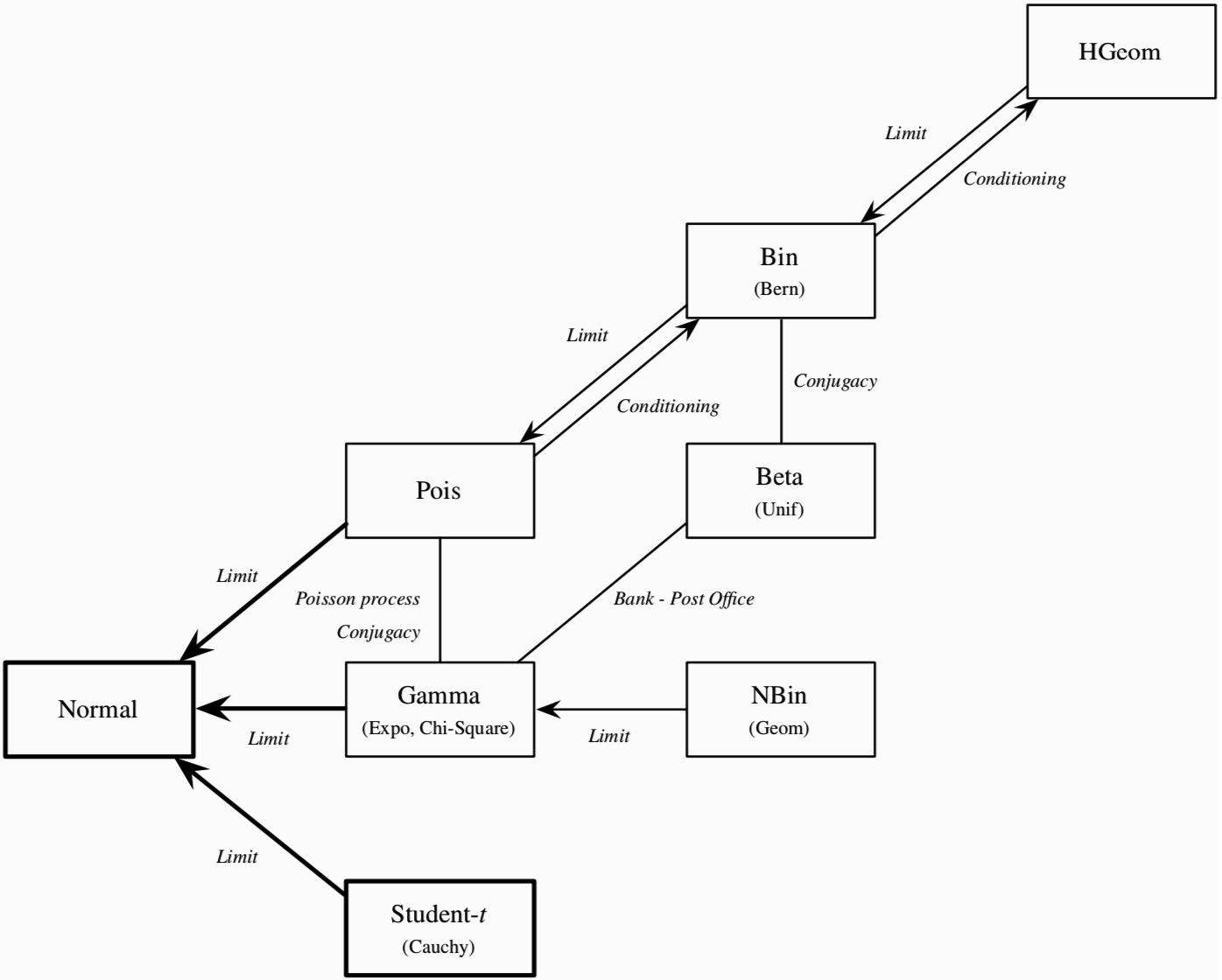
At the end of each chapter, the authors reflect on how newly introduced concepts relate to those from previous chapters. Spoiler alert: most probability distributions are related to each other when either conditioning on some event, or when taking the limit as $n \to \infty$. As Professor Blitzstein is fond of saying in the video lectures: “Conditioning is the soul of statistics”. The book incrementally builds the flowchart below, which we see in its complete form at the end of Chapter 10.
Does not assume prior knowledge
A common challenge with using material for self-study is that one’s own existing knowledge may not precisely match the known prerequisites of students taking the course which the textbook was written for. Rather than “assuming some calculus knowledge”, university instructors have the luxury of knowing the exact content of prerequisite courses in their own departments, and so can confidently skip reasoning steps which seem too basic to spell out explicitly.
Blitzstein & Hwang clearly go out of their way to decouple the course material from knowledge dependencies as much as possible. You will never hear the phrase It is trivial to prove… or read The proof of this theorem is left as an exercise… in this course. Whenever there is an unavoidable dependency on prior knowledge, the authors make explicit note of this fact, and reference the math appendix. The math appendix itself does a good job of cherry-picking useful prerequisite concepts—such as properties of functions, factorial and gamma functions, Taylor series, geometric series—and building intuition around them. For example: understanding how to apply a change-of-variables transformation to a multi-dimensional probability density function requires the concept of the Jacobian matrix, which itself requires a bit of multivariate calculus to understand fully. My calculus was a bit rusty to do the proof, but since I knew exactly what I was missing, it was straightforward to brush up on a few Khan Academy videos within an hour before continuing with the chapter.
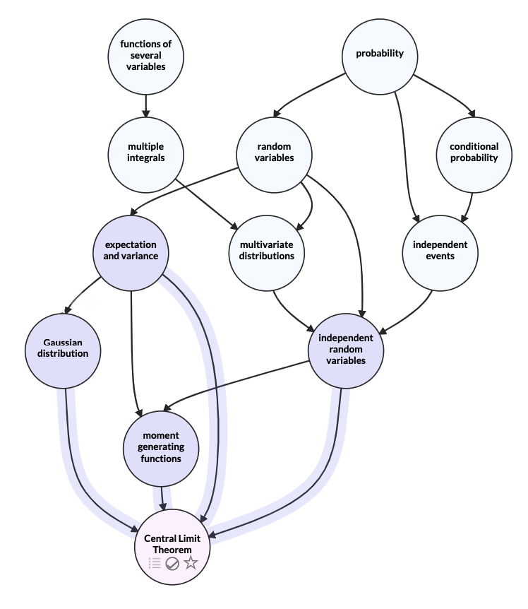
Although the author does not include a mindmap of concepts in the book, I found this Metacademy DAG for Central Limit Theorem (which is presented near the end of the book) to be a good approximation of how earlier concepts build up to concepts in the later chapters. Except for multiple integrals, there is an overall very little dependency on prior math knowledge.
The bad
Non-standard notation for some distributions
A matter of slight annoyance is that there are a few instances where the authors create their own parameterization of distributions which differ from the standard notation found outside of the book. For example, the notation for the Gamma distribution and its corresponding PDF is given as:
$$ \begin{aligned} Y &\sim \text{Gamma}(a, \lambda) \\\ f(y) &= \frac{1}{\Gamma(a)}(\lambda y)^a e^{-\lambda y} \frac{1}{y} \end{aligned} $$
Outside of the book, there are two typical parameterizations of the Gamma distribution: shape–scale or shape–rate. The shape–rate parameterization most closly matches the one we find in the book.
$$ \begin{aligned} X &\sim \text{Ga}(\alpha, \beta) \\\ f(x) &= \frac{\beta^\alpha}{\Gamma(\alpha)} x^{\alpha-1} e^{-\beta x} \end{aligned} $$
Why are they different? Well I’m sure that it is because the authors think their parameterization is more intuitive. If wikipedia can’t even agree on a single standard parameterization, why not introduce a third? I have mixed feelings here, because their choice of parameter $\lambda$ instead of $\beta$ actually is more intuitive, as it makes it more obvious how the Gamma distribution is closely related to the Exponential distribution, which shares the same rate parameter $\lambda$. But the form of the PDF makes it a bit tricky when referencing outside material alongside the textbook itself.
Another example of non-standard notation is around the presentation of the Geometric distribution. Outside of the course, this can refer to either the distribution of the number of Bernoulli trials before the first success (with support ${1, 2, 3, \ldots}$), or it can refer to the number of failures (with support ${0, 1, 2, \ldots }$). Blitzstein refers to the former as the First Success distribution, and the latter as the Geometric distribution. It is difficult to complain about not adhering to a common definition when the common definition itself is ambiguous. But this is something to keep in mind when referencing outside resources.
The ugly
There is no ugly. I struggled to even think of the above complaint about non-standard notation. This book is a gem, and I highly recommend it to anyone considering self-studying probability. In an ever-evolving data science field, it is difficult to predict which model or framework will be in vogue next year. But I think it’s a solid bet that probability will continue to play a central role in the field, and so there is a high ROI on investing the time to develop a solid understanding of the fundamental concepts this book covers.